
Metrics and evaluation
This challenge goal is focused, mainly, in evaluating how to deal with multirater annotations and how to exploit them.
Each CT has three different labels from three different experts with multiple classes: background (0), pancreas (1), kidney (2), liver (3).
Firstly, it is important to highlight that we will be working with three different regions (Figure 1):
- Foreground consensus area: region on which the three clinicians have agreed that belongs to de foreground.
- Background consensus area: region on which the three clinicians have agreed that belongs to de background.
- Dissensus area: region in which the three labelers do not agree.
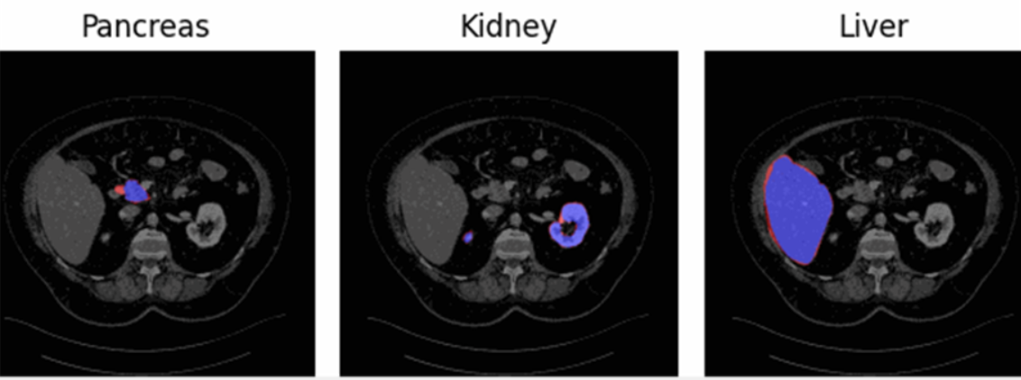
Figure 1 - Representation of the three regions for the three different organs. Consensus foreground area (blue), dissensus area (red), consensus background area (everything neither blue nor red).
For the evaluation of the challenge will have three main parts:
- Quality of the Segmentation
- Multi-rater Calibration
- Volume Assessment
1. Quality of the Segmentation and Uncertainty Consensus Assessment
The first metric we will use is the Dice Score (DSC) evaluation, which will assess only the consensus foreground and background areas for three classes: pancreas, kidney, and liver. This means that any predictions within the dissensus area will be ignored. False Positives (FP) can only occur in the consensus background area, and False Negatives (FN) can only occur in the consensus foreground area.
Additionally, we plan to study uncertainty within the consensus
regions. This study will be divided into two parts: the mean confidence
will be calculated separately for the consensus background ( ) and foreground areas
(
) and foreground areas
( ) of each class
(pancreas, kidney, and liver). Then, an average confidence metric per
class considering both consensus regions will be computed as defined in
Equation 1:
) of each class
(pancreas, kidney, and liver). Then, an average confidence metric per
class considering both consensus regions will be computed as defined in
Equation 1:

Equation 1 - Definition of the confidence assessment performed in the
consensus area ( ). being the consensus
background and being the foreground
areas.
). being the consensus
background and being the foreground
areas.
Finally, the mean of the three confidence values obtained per each class will be extracted to determine the overall confidence metric for evaluating uncertainty. The same approach will be applied to otbain the final averaged Dice Score.
2. Multi-rater Calibration
For the calibration study, the Expected Calibration Error (ECE) will be calculated, as defined in Equation 2. To maintain the multi-rater information, calibration will be computed for each prediction against each annotation, resulting in three ECE values, one per ground truth. Finally, to obtain a single calibration metric, the three ECEs will be equally averaged, thereby considering the information provided by each annotator.

Equation 2 - Expected Calibration Error (ECE). *  *being the bin in which
the sample *m** is,
*being the bin in which
the sample *m** is,  is the accuracy of such
bin,
is the accuracy of such
bin,  is the confidence of such
bin, and n the number of bins.*
is the confidence of such
bin, and n the number of bins.*
3. Volume Assessment
So far, the metrics we've discussed are not particularly relevant for real-world scenarios. To address this, we decided to explore the study of a biomarker, such as volume.
For this volume assessment, we adopted a different approach. First, we needed a method to retain information from the various annotations. Thus, we defined a gaussian Probabilistic Distribution Function (PDF) using the mean and standard deviation derived from computing the volume the three different annotations. Once the PDF was established, we then defined the corresponding Cumulative Distribution Function (CDF). See Figure 2.

Figure 2 - Probabilstic distribution function (first row) per organ. Cumulative distribution function (second row) per organ.
The predicted volume will be calculated by summing all the probabilistic values for the corresponding class from the probabilistic matrix provided by the participant. This method considers the model's uncertainty and confidence in its predictions when evaluating the volume.
For the evaluation of this section the Continuous Ranked Probability Score (CRPS) will be used, see Equation 3. The CRPS measures the average squared difference between a cumulative distribution and a predicted value.

Equation 3 - Continuous Ranked Pribability Score (CRPS).  being the PDF obtained
from the groundtruths (see Figure 2) and
being the PDF obtained
from the groundtruths (see Figure 2) and  being the heaviside
function of the volume calculated from the prediciton. For a graphical
representation of this equation see Figure 3.
being the heaviside
function of the volume calculated from the prediciton. For a graphical
representation of this equation see Figure 3.
For a clearer understanding, refer to Figure 3. On the left figure, the Gaussian PDF representing the volume of a structure (pancreas, kidney, or liver) is depicted in blue, derived from the mean and standard deviation computed from the three annotations. The red line represents the volume predicted by the model. On the right figure, the corresponding CDF of the aforementioned PDF is shown, with the predicted volume indicated in red. The orange line represents a Heaviside function derived from the predicted volume. The grey area represents what we calculate with the CRPS. A smaller grey area indicates that the predicted volume is closer to the mean, reflecting better performance.


Figure 3 - Visual example of a CRPS calculation.
In conclusion, by using CRPS, we will assess the accuracy of the probabilistic volume prediction relative to the ground truth volume probabilistic distribution.
Final Ranking
The final ranking will be defined by a combination of the four different rankins: Dice Score, Uncertainty, Calibration and Volume.